First practical session for "Introduction to image processing"
Bruno Galerne, Monday June 29, 2020
This is a step by step practical session to deal with images using Matlab.
The .m file to work with is here: https://www.idpoisson.fr/galerne/ed_images/tp1_intro_traitement_images.m
Download this file in a folder dedicated to the course and open matlab from there.
Contents
Open and display images
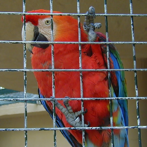
Download the image 'parrot.bmp' in your working folder: https://www.idpoisson.fr/galerne/ed_images/parrot.bmp
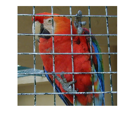
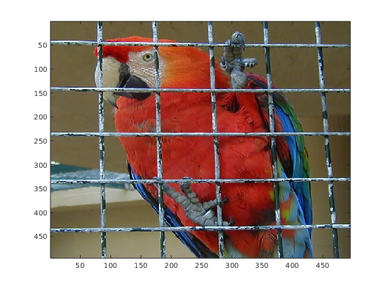
u = imread('parrot.bmp');

% size of u:

size(u)

% u is an RGB  image (3 chanels), each having size 495 x 495.
% store this values (to adapt to other images)
[M, N, nc] = size(u);
% M is the height, N is the width (matrix convention).

figure;
imshow(u);


% Note that with imshow you get a faithfull display:
%
% One pixel of the screen is one pixel of the image.
%
% This is not the case with the image function:

figure;
image(u)

% note that the aspect ratio is not preserved (fater parrot!)
ans =

   495   495     3
uint8 type
u = imread('parrot.bmp'); gives a matrix a type uint8.
uint8 type = integers between 0 and 255.
This is the 8-bits representation for pixel gray-level, but it is not possible to do computation with this :
x = uint8(250);
y = uint8(30);
s = y+x
d = y-x
m1 = (y+x)/2
m2 = y/2 + x/2
s =

  uint8

   255


d =

  uint8

   0


m1 =

  uint8

   128


m2 =

  uint8

   140
Conclusion: No processing with this type:
Always convert do double precision before any operation.
Only use uint8 before writing image file on disk.
Convert to double precision
u = double(imread('parrot.bmp'));

figure;
subplot(1,3,1);
imshow(u);
title('u double')
subplot(1,3,2);
imshow(uint8(u));
title('uint8(u)')
subplot(1,3,3);
imshow(u/255);
title('u/255')
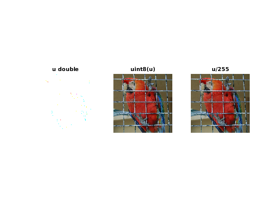
Warning:
For RGB images with double precision imshow assumes the convention of RGB colors in the cube [0,1]^3, while for uint8 type it is [0,255]^3.
RGB channels
Let us extract the chanels of an RGB image:
u = double(imread('parrot.bmp'))/255;
r = u(:,:,1); % always use semi-column otherwise display of all coefficient in the command window...
g = u(:,:,2);
b = u(:,:,3);

figure;
subplot(2,2,1);
imshow(u);
title('RGB image');
subplot(2,2,2);
imshow(r);
title('red chanel');
subplot(2,2,3);
imshow(g);
title('green chanel');
subplot(2,2,4);
imshow(b);
title('blue chanel');
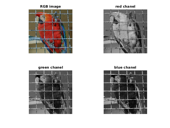
Here we visualize the chanels as gray-level images: dark is low and light is high. We can also create the RGB images with chanels equal to zero except for the displayed chanel
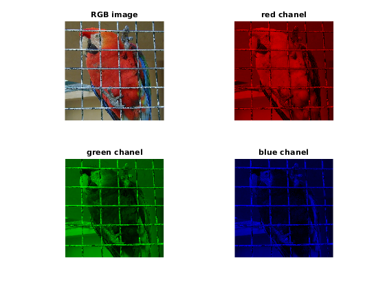
rRGB = zeros(size(u));
rRGB(:,:,1) = r;
EXERCICE: Do the same for green and blue chanels and obtain the display below. (for each exerice replace todo_**** with your command lines)
todo_RGBchanels
Convert an RGB image to a gray-level image
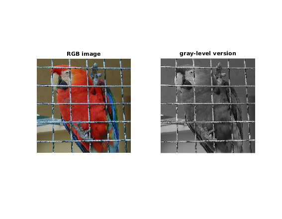
rgb2gray converts RGB values to grayscale values by forming a weighted sum of the R, G, and B components:
Y = 0.2989 * R + 0.5870 * G + 0.1140 * B
u = double(imread('parrot.bmp'))/255;
y = rgb2gray(u);

figure;
subplot(1,2,1)
imshow(u);
title('RGB image');
subplot(1,2,2)
imshow(y);
title('gray-level version');
Crop a subpart of the image:
One can extract subpart of images using matrix extraction. Let us recall the syntax on a small example
A = randi(99, [6,8]) % random matrix with integers between 1 and 99 of size 6x8.
B = A(2:4,3:6) % submatrix of A with lines 2 to 4 and columns 3 to 6.
A =

    98    10    51    21    71    21    45    86
    31    39    16    93    19    15    92    34
    63    80    78    33    16    45    14    39
    64    49    64    50    56    64    28    89
     8    83    84    92     2    75    68    61
    19    28    58    62    59    55    71    39


B =

    16    93    19    15
    78    33    16    45
    64    50    56    64
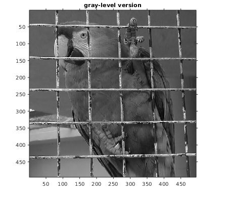
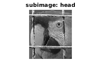
%Let us extract the parrot head in the grayscale image:
u = double(imread('parrot.bmp'))/255;
y = rgb2gray(u);

% First display image with axis:
figure;
imshow(y);
title('gray-level version');
axis on;

head = y(30:180, 70:200);
figure;
imshow(head);
title('subimage: head');
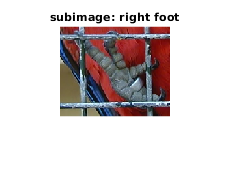
EXERCICE: Extract the right foot of the parrot from the RGB image and display the image:
todo_extract_subimgeRGB
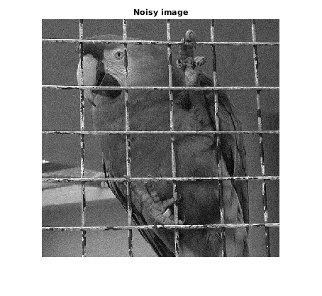
Add noise to an image
We will add noise to an image.
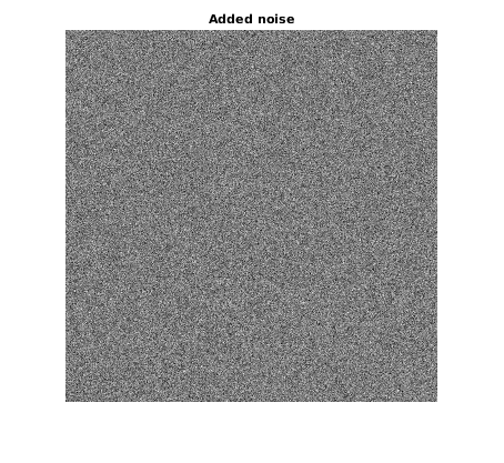
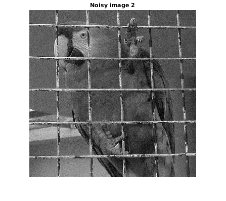
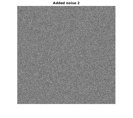
u = rgb2gray(double(imread('parrot.bmp'))/255);

% add Gaussian noise:
m = 0;
sigma = 10/255;
unoisy = imnoise(u,'gaussian', m, sigma^2);
n = unoisy-u;

figure;
imshow(unoisy)
title('Noisy image');
drawnow

figure;
imshow(n,[])
title('Added noise');
EXERCICE: Obtain a similar Gaussian noise using the randn function (see help)
todo_add_gaussian_noise
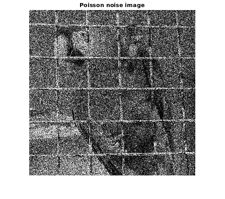
Now, let's generate Poisson noise: Each pixel (i,j) is a Poisson variable with mean/variance c*u(i,j).
c = 5;
upnoisy = random('Poisson', u*c)/c; % division by c to keep original range

figure;
imshow(upnoisy)
title('Poisson noise image');
drawnow

figure;
imshow(upnoisy-u,[])
title('Difference');
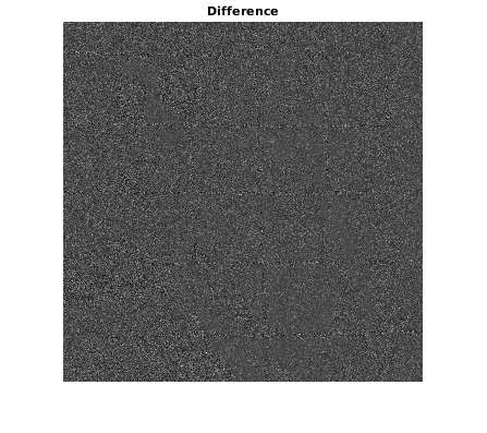
Observe that the noise has more variance in ligth arrays than in Dark ones.
Image Quantization
Image quantization consists in reducing the set of gray levels used to represent the image. This operation is useful for displaying an image u on a screen that supports a smaller number of colors (this is needed with a standard screen if u is coded on more than 8 bits per chanel).
Uniform quantization consists in dividing the set of 256 levels

into K < 256 regions.
u = rgb2gray(double(imread('parrot.bmp'))/255);

K = 20;

% for images having gray-levels in [0,1]:
uquant = (floor(u*(K-1)+0.5))/(K-1);

figure;
subplot(1,2,1)
imshow(u);
title('gray level');
subplot(1,2,2)
imshow(uquant);
title(['Quantized, K = ', num2str(K)]);
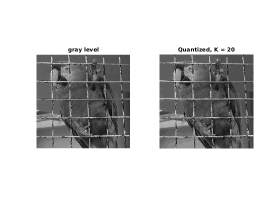
QUESTION: For which value of K do you start to see a difference with the original image ?
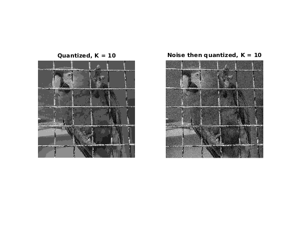
Dithering
Dithering consists in adding intentionnally noise to an image before quantization, in order to perceptually hide the quantization effects.
EXERCICE:
With a quantization of K=10, compare the quantized result of u and u corrupted with additional Gaussian white noise. For which range of standard deviation do you think the result is more pleasant?
todo_dithering
Credits:
Some parts of this practical session are inspired by: Julie Delon's "Introduction to image processing - Radiometry":
http://w3.mi.parisdescartes.fr/~jdelon/enseignement/tp_image/org/TP_radiometrie.html