Second practical session for "Introduction to image processing"

Bruno Galerne, Friday June 18, 2021

This is a step by step practical session to deal with images using Matlab.

The .m file to work with is here: https://www.idpoisson.fr/galerne/ed_images/tp2_intro_traitement_images.m

Download this file in a folder dedicated to the course and open matlab from there.

Image histogram
Histogram stretching:
Logarithmic contrast change:
Histogram Equalization:
Histogram matching:
Midway histogram:
Local Laplacian filtering of image
Denoising algorithms:
Credits:

Image histogram

Download the images in your working folder:

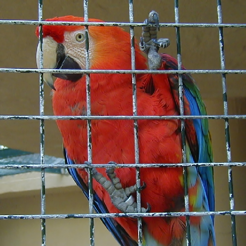
https://www.idpoisson.fr/galerne/ed_images/parrot.bmp

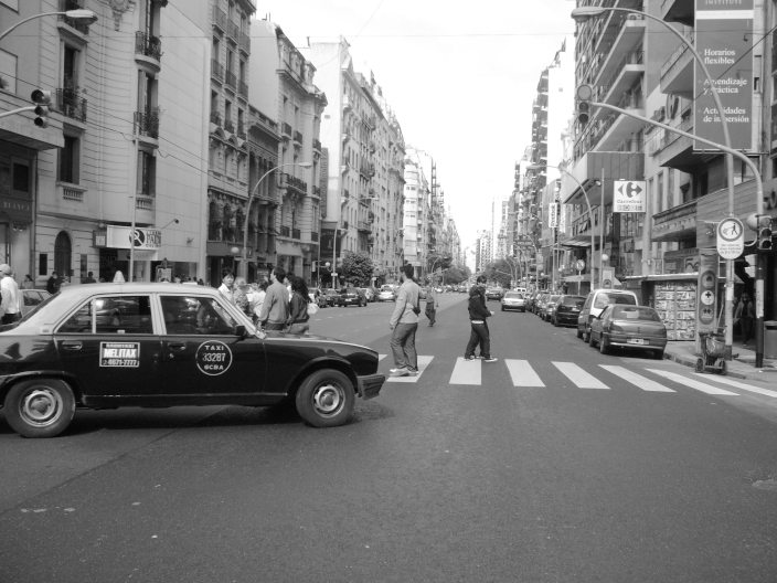
https://www.idpoisson.fr/galerne/ed_images/buenosaires3.bmp

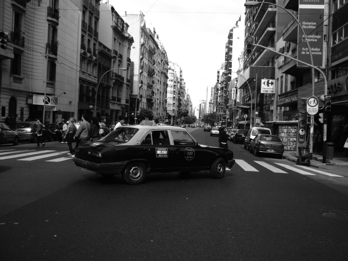
https://www.idpoisson.fr/galerne/ed_images/buenosaires4.bmp

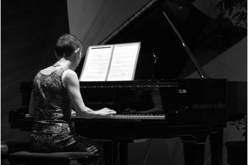
https://www.idpoisson.fr/galerne/ed_images/piano.png

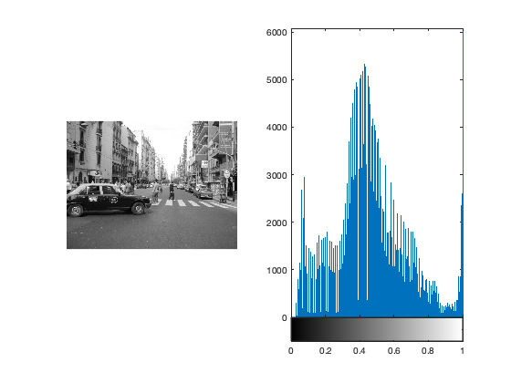
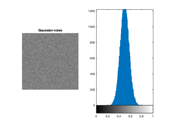
u = rgb2gray(double(imread('buenosaires3.bmp'))/255);

figure;
subplot(1,2,1);
imshow(u);
subplot(1,2,2);
imhist(u,256);


gn = 0.5 + 20/255*randn(256,256);

figure;
subplot(1,2,1);
imshow(gn);
title('Gaussian noise');
subplot(1,2,2);
imhist(gn,256);

Histogram stretching:

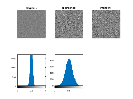
Histogram stretching consists in applying an affine contrast change to map the minimal gray-level to 0 and the maximal gray-level to 1 (or 255).

EXERCISE compute the image ustretch = a * (u - b) (with constants a and b to determine on paper) such that min(ustretch(:)) = 0 and max(ustretch(:)) = 1

u = 0.5 + 10/255*randn(256,256);

todo_stretching

Remark: Stretching is performed with the option [] in imshow(u,[]) check that your result is consistant

figure;
subplot(2,3,1);
imshow(u);
title('Original u');
subplot(2,3,2);
imshow(ustretch);
title('u streched');
subplot(2,3,3);
imshow(u,[]);
title('imshow []');
subplot(2,3,4);
imhist(u,256);
subplot(2,3,5);
imhist(ustretch,256);

Logarithmic contrast change:

Linear stretching is used to visualized any data, possibly with negative values (as we did for noise images, difference between two images, etc.).

Sometimes when values have different order of magnitudes, stretching is not sufficient to visualize data.

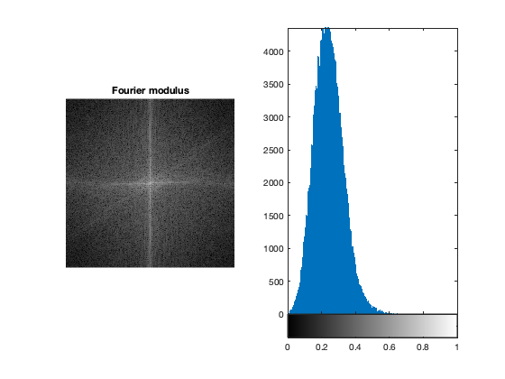
Here is an example with the modulus of the discrete Fourier transform of an image:

u = rgb2gray(double(imread('parrot.bmp'))/255);
mdftu = abs(fftshift(fft2(u)));


figure;
subplot(1,2,1);
imshow(mdftu,[]);
title('Fourier modulus');
subplot(1,2,2);
imhist(mdftu/max(mdftu(:)),256);

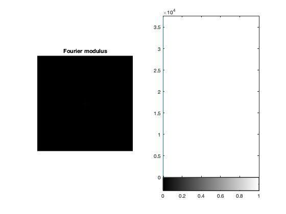
At first inspection the image is black with one pixel at the center... EXERCISE:

1. Apply g(x) = log(1+x) to mdftu and redo the visualization.

2. Explain why at the begining the image was black with one pixel at the center.

todo_logcontrast

Histogram Equalization:

Histogram Equalization consists in flattening an histogram to obtain

J = histeq(I,n) transforms the grayscale image I, returning in J an grayscale image with n discrete gray levels. A roughly equal number of pixels is mapped to each of the n levels in J, so that the histogram of J is approximately flat. The histogram of J is flatter when n is much smaller than the number of discrete levels in I.

u = rgb2gray(double(imread('parrot.bmp'))/255);

v = histeq(u,256);

figure;
subplot(2,2,1);
imshow(u);
subplot(2,2,2);
imhist(u,256);
subplot(2,2,3);
imshow(v);
subplot(2,2,4);
imhist(v,256);

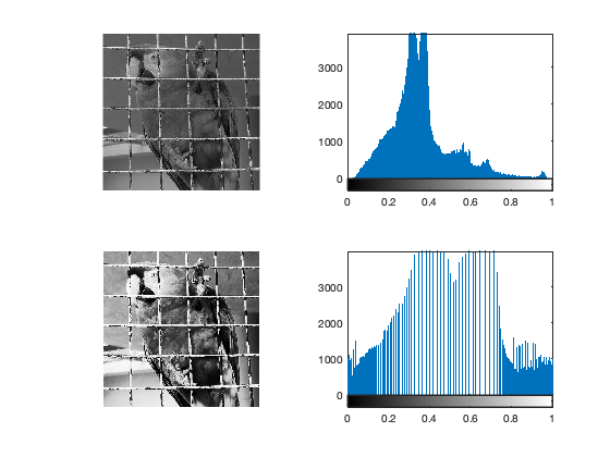
EXERCISE: Try this algorithm on piano.png. What do you observe? Can you explain the artefact?

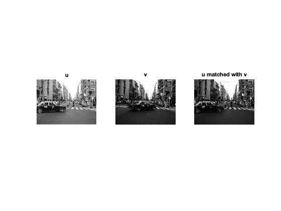
Histogram matching:

u = rgb2gray(double(imread('buenosaires3.bmp'))/255);
v = rgb2gray(double(imread('buenosaires4.bmp'))/255);

EXERCISE: program histogram matching by

1. sort the array u(:) (see 'help sort')

2. sort the array v(:)

3. affect to the k-th pixel of u (for the order of gray-level) the gray-level of the k-th pixel of v. (you may need to use 'reshape')

4. Display u, v and the new image (say uhistv)

If you find this too difficult, you can look at the solution here: https://www.idpoisson.fr/galerne/ed_images/todo_histmatching.m

todo_histmatching

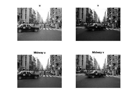
Midway histogram:

In the above hisogram matching, one image is favored. In may be better to use a compromise histogram. This is the goal of the midway histogram.

EXERCISE (optional) compute the midway histogram:

1. sort the array u(:)

2. sort the array v(:)

3. u_midway: affect to the k-th pixel of u (for the order of gray-level) the average gray-level of the k-th pixel of u and the k-th pixel of v. (you may need to use 'reshape')

4. Same for v_midway

5. Display u, v and the 2 new images u_midway and v_midway

todo_midway

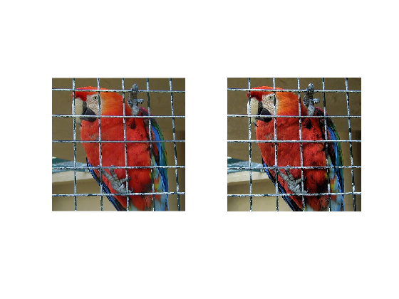
Local Laplacian filtering of image

EXERCISE: Try the function locallapfilt on the parrot image. Propose parameters that increase the local contrast while being faithful to the original image.

u = imread('parrot.bmp');
v=locallapfilt(u,0.9,0.8);

figure;
subplot(1,2,1);
imshow(u);

subplot(1,2,2);
imshow(v);

Denoising algorithms:

EXERCISE: Look at the following functions for denoising:

- imgaussfilt

- medfilt2

- imbilatfilt

- imnlmfilt

Compare them with three experiments: One with a small amount of Gaussian noise (sigma = 4/255), one with a large amount of Gaussian noise (sigma = 20/255), and one with impulse noise of 5%. Use the input grayscale image of your choice (one of yours would be nice, but use images of moderate size (eg a crop of an HD image)). Impulse noise means that a percentage of gray level is just random. You can extract randomly p% of pixels by applying a random permutation (randperm function) and extract the first p%.

Remark: For a near state of the art denoising alorithm that can be tried online:

The Noise Clinic: a Blind Image Denoising Algorithm Marc Lebrun, Miguel Colom, Jean-Michel Morel https://www.ipol.im/pub/art/2015/125/

Credits:

Some parts of this practical session are inspired by: Julie Delon's "Introduction to image processing - Radiometry":

http://w3.mi.parisdescartes.fr/~jdelon/enseignement/tp_image/org/TP_radiometrie.html