Second practical session for "Introduction to image processing"

Bruno Galerne, Monday June 28, 2021

Link to the .m file:

https://www.idpoisson.fr/galerne/ed_images/tp3_intro_traitement_images.m

Download this file in a folder dedicated to the course and open matlab from there.

Download the images:
Discrete Fourier transform:
Low pass filter
Image sharpening
Image segmentation using histogram thresholding
imageSegmenter:
Credits:

Download the images:

https://www.idpoisson.fr/galerne/ed_images/image_sharpening.png

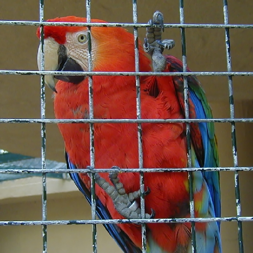
https://www.idpoisson.fr/galerne/ed_images/parrot.bmp

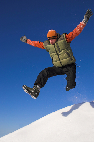
https://www.idpoisson.fr/galerne/ed_images/jump.jpg

Discrete Fourier transform:

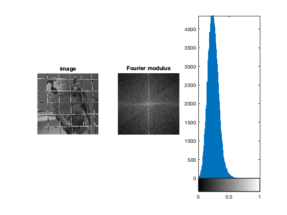
Recall from TP2:

u = rgb2gray(double(imread('parrot.bmp'))/255);
mdftu = abs(fftshift(fft2(u)));
logmdftu = log(1+mdftu);

figure;
subplot(1,3,1);
imshow(u);
title('image');
subplot(1,3,2);
imshow(logmdftu,[]);
title('Fourier modulus');
subplot(1,3,3);
imhist(logmdftu/max(logmdftu(:)),256);
drawnow

Low pass filter

Reproduce the low-pass filter demo in Matlab using the Parrot image (in grayscale) The code to produce a disk image is given below.

Discuss the different details that appear as the radius grows.

u = rgb2gray(double(imread('parrot.bmp'))/255);
% crop if odd size:
if mod(size(u,2),2) == 1
    u = u(1:end-1,:);
end
if mod(size(u,2),2) == 1
    u = u(:,1:end-1);
end

[M,N] = size(u);
radius = 100;
[Y,X] = meshgrid((-N/2):(N/2-1),(-M/2):(M/2-1));
D = X.^2+Y.^2; % distance to center at (M/2+1, N/2+1)
mask = (D <= radius^2);

figure
subplot(2,2,1)
imshow(X,[])
title('1st Fourier index');
subplot(2,2,2)
imshow(Y,[])
title('2nd Fourier index');
subplot(2,2,3)
imshow(D,[])
title('Distance to center');
subplot(2,2,4)
imshow(mask,[]);
title('Mask');

todo_low_pass_filter

% todo test image rectangulaire.

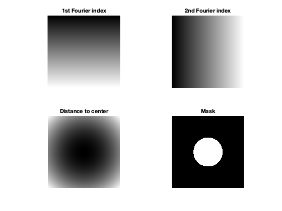
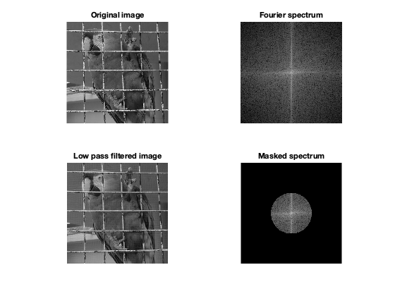
Image sharpening

Reproduce the experiment for image sharpening on the image 'image_sharpening.png'.

To do the smooth mask, apply a Gaussian convolution filter to the binary disk used above.

u = double(imread('image_sharpening.png'))/255;
figure;
imshow(u);

%TODO

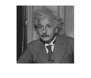
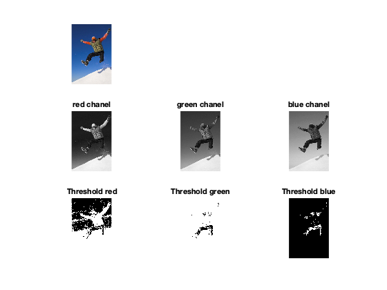
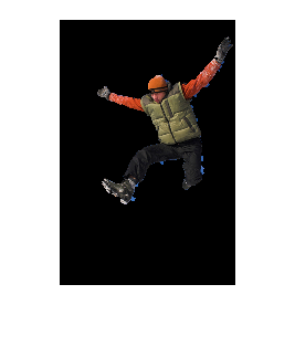
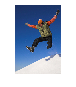
Image segmentation using histogram thresholding

Find the best chanel and best threshold for this channel to segment the man in the picture.

u = double(imread('jump.jpg'))/255;
r = u(:,:,1); % always use semi-column otherwise display of all coefficient in the command window...
g = u(:,:,2);
b = u(:,:,3);

tr = 30/255;
tg = 30/255;
tb = 30/255;

figure;
subplot(3,3,1);
imshow(u);

subplot(3,3,4);
imshow(r);
title('red chanel');
subplot(3,3,5);
imshow(g);
title('green chanel');
subplot(3,3,6);
imshow(b);
title('blue chanel');
subplot(3,3,7);
imshow(u(:,:,1)>tr);
title('Threshold red');
subplot(3,3,8);
imshow(u(:,:,2)>tg);
title('Threshold green');

subplot(3,3,9);
imshow(u(:,:,3)<tb);
title('Threshold blue');

imageSegmenter:

Try the imagesegmenter with the jump image and an image of your own. Send me the mask by email.

Use the "export" button.

Then use imwrite(uint8(255*maskedImage), 'segmented_result.png');

Command to execute: imageSegmenter(u); % save result after Export: % imwrite(uint8(255*maskedImage), 'segmented_result.png');

% my result:
figure;
imshow(imread('jump.jpg'));
figure;
imshow(imread('segmented_result.png'))

Credits:

Some parts of this practical session are inspired by: C. Deledalle course:

https://www.charles-deledalle.fr/pages/teaching.php

jump image from:

https://matlabtricks.com/post-35/a-simple-image-segmentation-example-in-matlab